15 May Support Vector Machine (SVM) Algorithm in Machine Learning
Support Vector Machine (SVM) is a powerful supervised machine learning algorithm used for both classification and regression tasks. It’s particularly effective in high-dimensional spaces and is based on the concept of finding an optimal hyperplane that best separates data points of different classes.
SVM is a supervised learning algorithm as it requires labeled training data to learn the decision boundaries. In this lesson, we will learn:
- How Support Vector Machine (SVM) Works
- Features of Support Vector Machine (SVM)
- Advantages of Support Vector Machine
- Disadvantages of Support Vector Machine
- Applications of Support Vector Machine
- When to Use Support Vector Machine
- When to Avoid Support Vector Machine
- Example 1: SVM for Classification with Python and Scikit Learn
- Example 2: SVM for Regression with Python and Scikit Learn
- Example 3: SVM for Classification with Plot
- Example 4: SVM for Regression with Plot
How Support Vector Machine (SVM) Works
For classification, SVM finds the optimal hyperplane that maximizes the margin between different classes. The data points closest to the hyperplane are called “support vectors.”
For regression, SVM tries to fit as many instances as possible within a margin around the predicted line while limiting margin violations.
Features of Support Vector Machine (SVM)
The following are the features of Support Vector Machine:
- Kernel Trick: SVM can use various kernel functions (linear, polynomial, RBF, sigmoid) to handle non-linear decision boundaries
- Classification and Regression: SVM can be used for both:
- Classification (SVC – Support Vector Classification)
- Regression (SVR – Support Vector Regression)
- Margin Maximization: Focuses on finding the decision boundary with maximum margin
- Effective in High Dimensions: Works well even when number of features exceeds number of samples
- Memory Efficient: Uses only support vectors for prediction, not the entire dataset
Advantages of Support Vector Machine
The following are the advantages of Support Vector Machine:
- Effective in high-dimensional spaces
- Versatile through kernel functions
- Robust against overfitting, especially in high-dimensional space
- Works well with clear margin of separation
- Memory efficient (only stores support vectors)
Disadvantages of Support Vector Machine
The following are the disadvantages of Support Vector Machine:
- Not suitable for very large datasets (slow training)
- Doesn’t perform well with noisy data or overlapping classes
- Requires careful tuning of hyperparameters (C, kernel choice, gamma)
- Less intuitive interpretation compared to decision trees
- Binary by nature (though extensions exist for multi-class)
Applications of Support Vector Machine
The following are the applications of Support Vector Machine:
- Text categorization
- Image classification
- Handwriting recognition
- Biological sciences (protein classification, cancer classification)
- Stock market prediction
- Face detection
When to Use Support Vector Machine
Let us see when to use Support Vector Machine:
- When you have a clear margin of separation
- For high-dimensional data
- When you need a model with good generalization
- For complex but small-to-medium-sized datasets
When to Avoid Support Vector Machine
Let us see when to avoid Support Vector Machine:
- With very large datasets (training can be slow)
- With noisy data or overlapping classes
- When you need probability estimates
- When interpretability is important
Example 1: SVM for Classification with Python and Scikit Learn
We are using the IRIS Dataset and achieving the following objective to classify IRIS flowers:
- Primary Goal:
- To classify iris flowers into one of three species (setosa, versicolor, virginica) based on their sepal and petal measurements.
- Key Steps & Objectives:
- Load Data: Use the Iris dataset (features: sepal length/width, petal length/width; target: species label).
- Train-Test Split: Divide data into 70% training and 30% testing to evaluate generalization.
- Model Selection: Use
SVC(Support Vector Classifier) with an RBF kernel to handle non-linear boundaries. - Hyperparameters:
C=1.0: Balances margin width vs. classification errors.gamma='scale': Controls kernel flexibility (auto-adjusted based on data variance).
- Evaluation:
- Accuracy: Measure overall correctness of predictions.
- Classification Report: Show precision, recall, and F1-score per class to assess per-species performance.
- Why SVM for Classification?
- Iris data has clear margins between classes.
- SVM maximizes the separation boundary, making it robust for small, high-dimensional datasets.
Here are the steps:
Step 1: Import the required libraries
from sklearn import datasets
from sklearn.model_selection import train_test_split
from sklearn.svm import SVC
from sklearn.metrics import accuracy_score, classification_report
Step 2: Load iris dataset
iris = datasets.load_iris()
X = iris.data
y = iris.target
Step 3: Split data
X_train, X_test, y_train, y_test = train_test_split(X, y, test_size=0.3, random_state=42)
Step 4: Create SVM classifier
svm_classifier = SVC(kernel='rbf', C=1.0, gamma='scale') # RBF kernel
svm_classifier.fit(X_train, y_train)
Step 5: Predict
y_pred = svm_classifier.predict(X_test)
Step 6: Evaluate
print("Accuracy:", accuracy_score(y_test, y_pred))
print("\nClassification Report:\n", classification_report(y_test, y_pred))
Output

Example 2: SVM for Regression with Python and Scikit Learn
We are using the Diabetes Dataset and achieving the following objective to predict the progression of diabetes:
- Primary Goal:
- To predict the progression of diabetes (a continuous value) based on patient features (age, BMI, blood pressure, etc.).
- Key Steps & Objectives:
- Load Data: Use the Diabetes dataset (features: 10 physiological variables; target: disease progression score).
- Feature Scaling: Standardize features (critical for SVM regression to ensure equal weighting).
- Train-Test Split: 70-30 split for reliable performance estimation.
- Model Selection: Use
SVR(Support Vector Regressor) with a linear kernel (assuming linear relationships). - Hyperparameters:
C=1.0: Penalty for deviations beyond the margin.epsilon=0.1: Defines the “tolerance margin” where errors are ignored (larger = more tolerant).
- Evaluation:
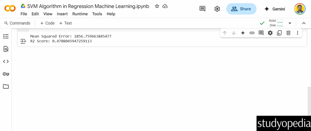
- Mean Squared Error (MSE): Quantifies average prediction error (lower = better).
- R² Score: Measures how well the model explains variance in the target (1 = perfect fit).
- Why SVM for Regression?
- Effective when relationships between features and target are complex but not highly noisy.
epsilonallows control over the margin of error, useful for medical predictions where approximations are acceptable.
Here are the steps:
Step 1: Import the required libraries
from sklearn import datasets
from sklearn.model_selection import train_test_split
from sklearn.svm import SVR
from sklearn.metrics import mean_squared_error, r2_score
from sklearn.preprocessing import StandardScaler
Step 2: Load diabetes dataset
diabetes = datasets.load_diabetes()
X = diabetes.data
y = diabetes.target
Step 3: Split data
X_train, X_test, y_train, y_test = train_test_split(X, y, test_size=0.3, random_state=42)
Step 4: Scale features
scaler = StandardScaler()
X_train = scaler.fit_transform(X_train)
X_test = scaler.transform(X_test)
Step 5: Create SVM regressor
svm_regressor = SVR(kernel='linear', C=1.0, epsilon=0.1) # Linear kernel
svm_regressor.fit(X_train, y_train)
Step 6: Predict
y_pred = svm_regressor.predict(X_test)
Step 7: Evaluate
print("Mean Squared Error:", mean_squared_error(y_test, y_pred))
print("R2 Score:", r2_score(y_test, y_pred))
Output
Comparing both examples
| Aspect | Classification (SVC) | Regression (SVR) |
|---|---|---|
| Goal | Classify discrete labels (e.g., flower species). | Predict continuous values (e.g., disease progression). |
| Dataset Used | Iris (4 features, 3 classes). | Diabetes (10 features, continuous target). |
| Key Parameter | kernel='rbf' (for non-linear boundaries). | epsilon=0.1 (error tolerance margin). |
| Evaluation Metrics | Accuracy, precision, recall. | MSE, R² score. |
Example 3: SVM for Classification with Plot
Objective: Visualize the decision boundary for iris classification (2D projection for simplicity).
Here are the steps:
Step 1: Import the required libraries
import numpy as np
import matplotlib.pyplot as plt
from sklearn import datasets
from sklearn.svm import SVC
from sklearn.decomposition import PCA
Step 2: Load iris data
iris = datasets.load_iris()
X = iris.data[:, :2] # Use only 2 features (sepal length/width) for visualization
y = iris.target
Step 3: Train SVM
svm = SVC(kernel='linear', C=1.0)
svm.fit(X, y)
Step 4: Create a meshgrid for decision boundary
x_min, x_max = X[:, 0].min() - 1, X[:, 0].max() + 1
y_min, y_max = X[:, 1].min() - 1, X[:, 1].max() + 1
xx, yy = np.meshgrid(np.arange(x_min, x_max, 0.02),
np.arange(y_min, y_max, 0.02))
Z = svm.predict(np.c_[xx.ravel(), yy.ravel()])
Z = Z.reshape(xx.shape)
Step 5: Plot
plt.figure(figsize=(10, 6))
plt.contourf(xx, yy, Z, alpha=0.8, cmap=plt.cm.Paired)
plt.scatter(X[:, 0], X[:, 1], c=y, edgecolors='k', cmap=plt.cm.Paired)
plt.xlabel('Sepal Length (cm)')
plt.ylabel('Sepal Width (cm)')
plt.title('SVM Decision Boundary (Iris Classification)')
plt.colorbar(label='Class')
plt.show()
Output
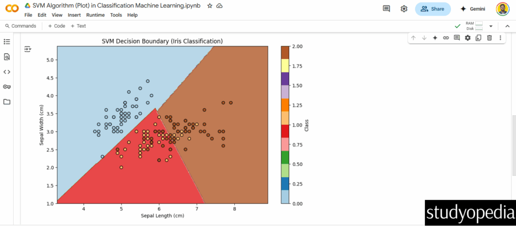
Key Plot Features:
-
Decision Boundary: Shows regions where the model predicts each class.
-
Support Vectors: Points near the boundary (not explicitly marked here but critical to SVM).
-
Objective: Demonstrate how a linear kernel separates the classes in 2D feature space.
Example 4: SVM for Regression with Plot
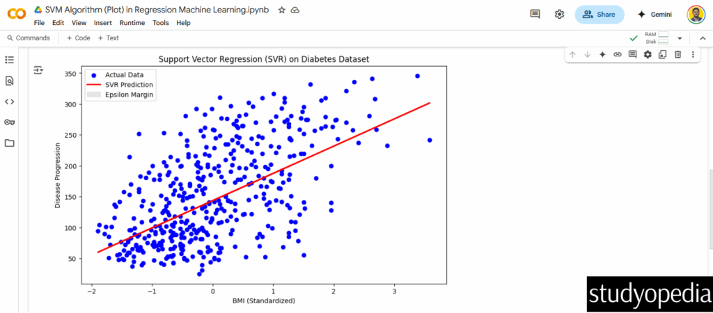
Objective: Visualize how SVR fits a continuous target (diabetes progression).
Here are the steps:
import numpy as np
import matplotlib.pyplot as plt
from sklearn import datasets
from sklearn.svm import SVR
from sklearn.preprocessing import StandardScaler
Step 2: Load diabetes data
diabetes = datasets.load_diabetes()
X = diabetes.data[:, np.newaxis, 2]  # Use only BMI feature (column index 2)
y = diabetes.target
Step 3: Scale data (critical for SVR)
scaler = StandardScaler()
X_scaled = scaler.fit_transform(X)
Step 4: Train SVR model
svr = SVR(kernel='linear', C=1.0, epsilon=0.2)
svr.fit(X_scaled, y)
Step 5: Predict
y_pred = svr.predict(X_scaled)
Step 6: Plot results
plt.figure(figsize=(10, 6))
plt.scatter(X_scaled, y, color='blue', label='Actual Data')
plt.plot(X_scaled, y_pred, color='red', linewidth=2, label='SVR Prediction')
plt.fill_between(X_scaled.flatten(),
                 y_pred - svr.epsilon,
                 y_pred + svr.epsilon,
                 color='gray', alpha=0.2, label='Epsilon Margin')
plt.xlabel('BMI (Standardized)')
plt.ylabel('Disease Progression')
plt.title('Support Vector Regression (SVR) on Diabetes Dataset')
plt.legend()
plt.show()
Output
If you liked the tutorial, spread the word and share the link and our website Studyopedia with others.
For Videos, Join Our YouTube Channel: Join Now
Read More:
No Comments