14 May Naive Bayes Algorithm

Naive Bayes is a supervised learning algorithm. It is a probabilistic machine learning algorithm based on Bayes’ Theorem with an assumption of independence among predictors (features). It is primarily used for classification tasks, not regression. In this lesson, we will learn:

• Features of Naive Bayes
• Types of Naive Bayes Algorithms
• Advantages of Naive Bayes Algorithms
• Disadvantages of Naive Bayes Algorithms
• Example: Spam Email Classification with Naive Bayes

Features of Naive Bayes

The following are the features of the Naive Bayes algorithm:

1. Probabilistic Model: Calculates the probability of a data point belonging to a class.
2. “Naive” Assumption: Assumes features are independent of each other (though this is rarely true in real-world data).
3. Fast & Efficient: Works well even with large datasets.
4. Low Computational Cost: Requires less training time compared to complex models.
5. Works Well with High-Dimensional Data: Such as text classification (e.g., spam detection).

Types of Naive Bayes Algorithms

The following are the types of the Naive Bayes algorithm:

1. Gaussian Naive Bayes: Assumes continuous features follow a normal distribution.
2. Multinomial Naive Bayes: Used for discrete counts (e.g., text classification with word frequencies).
3. Bernoulli Naive Bayes: For binary/boolean features (e.g., presence/absence of words).

Advantages of Naive Bayes Algorithms

The following are the advantages of the Naive Bayes algorithm:

• Simple & easy to implement
• Performs well with small datasets
• Handles High-Dimensional data well (e.g., NLP tasks)
• Less prone to Overfitting (due to simplicity)
• Works well with Categorical features

Disadvantages of Naive Bayes Algorithms

The following are the disadvantages of the Naive Bayes algorithm:

• Strong Independence Assumption (Features are rarely independent in reality)
• Zero-Frequency Problem: If a category in test data was not seen in training, it assigns zero probability (can be fixed using smoothing techniques).
• Not Suitable for Complex Relationships (Performs poorly if features are highly correlated)

Example: Spam Email Classification

Let us see the Naive Bayes Python Implementation example:

• Problem: Classify emails as “Spam” (1) or “Not Spam” (0) based on words.
• What we’ll do: We’ll use the scikit-learn library to implement Naive Bayes for spam email classification.
• Dataset Used: We’ll create a simple dataset with emails and labels (0 = Not Spam, 1 = Spam).

Steps:

1. Import Libraries
2. Prepare Dataset (Text → Numerical Features using CountVectorizer)
3. Train-Test Split
4. Train Naive Bayes Model (MultinomialNB)
5. Evaluate Model (Accuracy, Confusion Matrix)

Here are the steps with the code snippets:

Step 1: Import Required Libraries

Step 5. Train the Naive Bayes Model

Step 6. Make Predictions & Evaluate Model

Output till now:

Step 7. Test on a New Email

Complete Output

The following is the output. We ran the code on Google Colab:

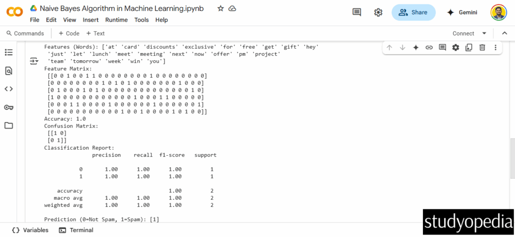
The above screenshot shows the output is:

Key Takeaways from the Code

• Text Preprocessing: CountVectorizer converts text into word counts.
• MultinomialNB: Best for discrete word counts (text classification).
• High Accuracy: Works well even with small datasets.
• Real-World Use Case: Used in spam filters, sentiment analysis, and document categorization.

---

If you liked the tutorial, spread the word and share the link and our website Studyopedia with others.

---

For Videos, Join Our YouTube Channel: Join Now

---

Read More:

• Model Evaluation Terminologies
• Confusion Matrix in Machine Learning
• Accuracy in Machine Learning
• Precision in Machine Learning
• Recall in Machine Learning
• F1 Score in Machine Learning
• Statistics for ML Tutorial
• Deep Learning Tutorial