15 May K-Nearest Neighbors (KNN) Algorithm

The K-Nearest Neighbors (KNN) algorithm is a simple, non-parametric, and instance-based supervised learning algorithm used for classification and regression tasks in machine learning. It works by finding the K most similar training examples (neighbors) to a new data point and making predictions based on their labels (for classification) or values (for regression).

In this lesson, we will learn:

• Features of KNN
• Advantages of KNN
• Disadvantages of KNN
• Applications of KNN
• Example 1: K-Nearest Neighbors (KNN) for Classification in Python
• Example 2: K-Nearest Neighbors (KNN) for Regression in Python

Features of KNN

The following are the features of KNN:

1. Lazy Learning Algorithm – KNN does not learn a model during training; instead, it memorizes the entire dataset and computes predictions at runtime.
2. Distance-Based – Uses distance metrics (Euclidean, Manhattan, Minkowski, etc.) to find the nearest neighbors.
3. Hyperparameter (K) – The number of neighbors (K) must be chosen carefully (odd number for classification to avoid ties).
4. No Training Phase – Unlike other ML algorithms, KNN does not require explicit training.
5. Works for Both Classification & Regression
   • Classification: Predicts the majority class among K neighbors.
   • Regression: Predicts the average (or weighted average) of K neighbors.

Advantages of KNN

The following are the advantages of KNN:

• Simple & Easy to Implement – No complex mathematical modeling required.
• No Training Phase – Works directly on stored data.
• Adapts to New Data Easily – New data points can be added without retraining.
• Works Well for Small Datasets – Effective when data is not too large.
• Versatile – Can be used for both classification and regression.

Disadvantages of KNN

The following are the disadvantages of KNN:

• Computationally Expensive – Requires calculating distances for all training points for each prediction.
• Sensitive to Irrelevant Features – Needs feature scaling (normalization/standardization).
• Struggles with High-Dimensional Data – “Curse of dimensionality” affects performance.
• Choice of K is Crucial – Small K → Overfitting, Large K → Underfitting.
• Memory Intensive – Stores the entire dataset.

Applications of KNN

The following are the applications of KNN:

• Medical Diagnosis (Disease classification based on symptoms)
• Recommendation Systems (Suggesting products based on similar users)
• Image Recognition (Handwritten digit classification)
• Finance (Credit scoring, fraud detection)
• Geographical Data Analysis (Predicting weather conditions)

Example 1: K-Nearest Neighbors (KNN) for Classification in Python

Here’s a step-by-step implementation of the KNN algorithm for classification using Python and scikit-learn. We’ll use the famous Wine dataset for this example:

• Objective: Classify wine into 3 categories based on chemical properties.
• Workflow: Data loading → Preprocessing → Training → Evaluation → Visualization

Steps:

Step 1: Import libraries

import numpy as np
import matplotlib.pyplot as plt
from sklearn.datasets import load_wine
from sklearn.model_selection import train_test_split
from sklearn.preprocessing import StandardScaler
from sklearn.neighbors import KNeighborsClassifier
from sklearn.metrics import classification_report, accuracy_score
from mlxtend.plotting import plot_decision_regions  # Requires mlxtend: !pip install mlxtend

Step 2: Load Dataset

wine = load_wine()
X, y = wine.data, wine.target
feature_names = wine.feature_names

Step 3: Display Dataset Info

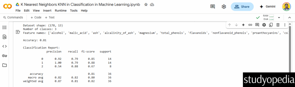
print(f"Dataset shape: {X.shape}")
print(f"Number of classes: {len(np.unique(y))}")
print(f"Feature names: {feature_names}")

Step 4: Select 2 most important features for visualization (alcohol & malic_acid)

X_2d = X[:, [0, 1]] # First two features

Step 5: Scale features

scaler = StandardScaler()
X_scaled = scaler.fit_transform(X_2d)

Step 6: Split data

X_train, X_test, y_train, y_test = train_test_split(
X_scaled, y, test_size=0.2, random_state=42
)

Step 7: Train KNN (K=5)

knn = KNeighborsClassifier(n_neighbors=5)
knn.fit(X_train, y_train)

Step 8: Predictions

y_pred = knn.predict(X_test)

Step 9: Metrics

print(f"\nAccuracy: {accuracy_score(y_test, y_pred):.2f}")
print("\nClassification Report:")
print(classification_report(y_test, y_pred))

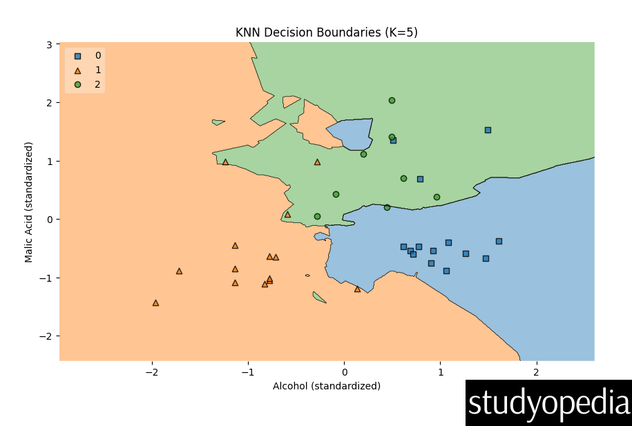
Step 10: Plot decision boundaries

plt.figure(figsize=(10, 6))
plot_decision_regions(X_test, y_test, clf=knn, legend=2)
plt.xlabel("Alcohol (standardized)")
plt.ylabel("Malic Acid (standardized)")
plt.title("KNN Decision Boundaries (K=5)")
plt.show()

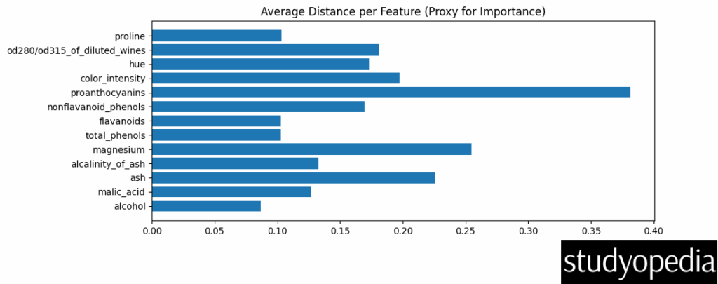
Step 11: Feature importance plot (using mean distance impact)

feature_importance = np.mean(knn.kneighbors(X_scaled)[0], axis=1)
plt.figure(figsize=(10, 4))
plt.barh(feature_names, feature_importance[:len(feature_names)])
plt.title("Average Distance per Feature (Proxy for Importance)")
plt.show()

Output

The output generates the following visualizations also:

Decision Boundary Plot:

1. • Shows how KNN classifies based on alcohol and malic acid content
   • Each colored region represents a wine class

Feature Importance:

• • Proxies importance via average neighbor distance per feature
  • Higher bars = more separation power

Example 2 K-Nearest Neighbors (KNN) for Regression in Python

Here’s the complete Python example for KNN Regression using the California Housing dataset, with all necessary steps from data loading to evaluation.

We’re predicting median house values (continuous numbers) based on neighborhood features.

Steps:

Step 1: Import required libraries

from sklearn.datasets import fetch_california_housing
from sklearn.model_selection import train_test_split
from sklearn.preprocessing import StandardScaler
from sklearn.neighbors import KNeighborsRegressor
from sklearn.metrics import mean_squared_error, r2_score
import matplotlib.pyplot as plt
import numpy as np # Import numpy for sqrt

Step 2: Load dataset

housing = fetch_california_housing()
X, y = housing.data, housing.target
feature_names = housing.feature_names

Step 3: Display dataset info

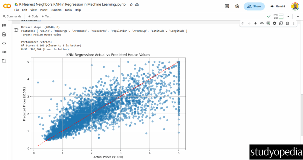
print(f"Dataset shape: {X.shape}")
print(f"Features: {feature_names}")
print(f"Target: Median House Value")

Step 4: Feature scaling (critical for KNN)

scaler = StandardScaler()
X_scaled = scaler.fit_transform(X)

Step 5: Split into train-test (80-20)

X_train, X_test, y_train, y_test = train_test_split(
X_scaled, y, test_size=0.2, random_state=42
)

Step 6: Initialize and train KNN regressor (K=5)

knn_reg = KNeighborsRegressor(n_neighbors=5)
knn_reg.fit(X_train, y_train)

Step 7: Predictions

y_pred = knn_reg.predict(X_test)

Step 8: Evaluation metrics

r2 = r2_score(y_test, y_pred)

Step 9: Calculate RMSE by taking the square root of the Mean Squared Error

rmse = np.sqrt(mean_squared_error(y_test, y_pred))

print(f"\nPerformance Metrics:")
print(f"R² Score: {r2:.3f} (Closer to 1 is better)")
print(f"RMSE: ${rmse*100000:,.0f} (Lower is better)")

Step 10: Plot actual vs predicted values

plt.figure(figsize=(10, 6))
plt.scatter(y_test, y_pred, alpha=0.5)
plt.plot([y.min(), y.max()], [y.min(), y.max()], 'r--')
plt.xlabel("Actual Prices ($100k)")
plt.ylabel("Predicted Prices ($100k)")
plt.title("KNN Regression: Actual vs Predicted House Values")
plt.grid()
plt.show()

Output

---

If you liked the tutorial, spread the word and share the link and our website Studyopedia with others.

---

For Videos, Join Our YouTube Channel: Join Now

---

Read More:

• Naive Bayes Algorithm
• Random Forest Algorithm
• What is Model Evaluation
• Model Evaluation Terminologies
• Confusion Matrix in Machine Learning
• Accuracy in Machine Learning
• Precision in Machine Learning
• Recall in Machine Learning
• F1 Score in Machine Learning