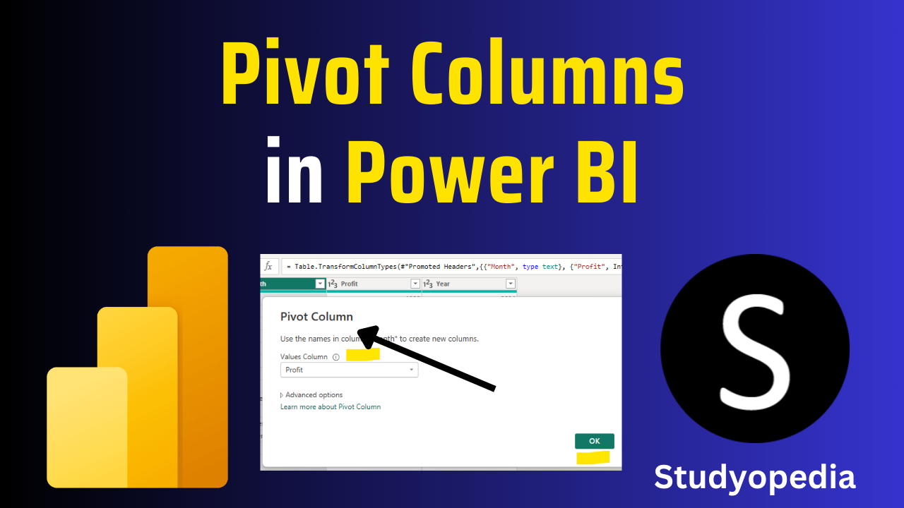
10 Sep Power BI – Pivot columns
Pivot on columns in Power BI means converting columns to rows. We will first get the data and then perform the pivot column operation.
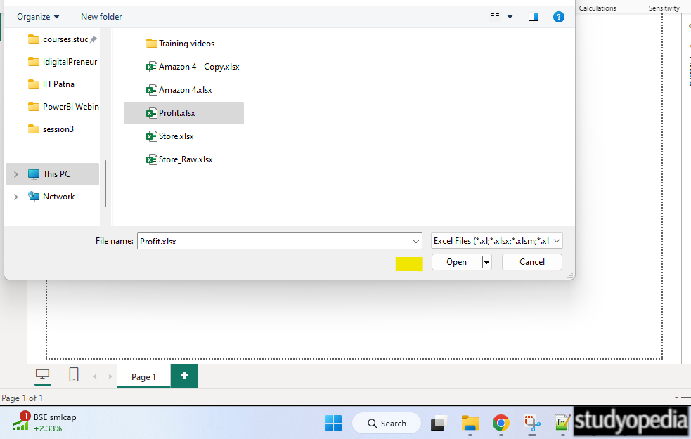
Input File: Profit.xlsx
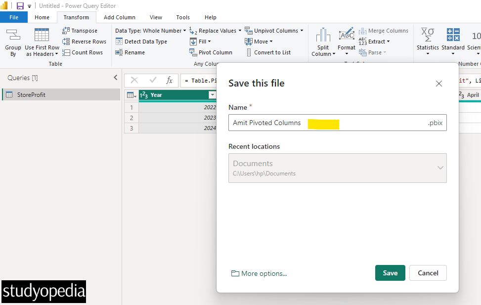
Output Saved as: Amit Pivoted Column.pbix
Click Get Data and select Excel Workbook. We have an Excel file named Profit.xlsx. Select and click Open to add it:
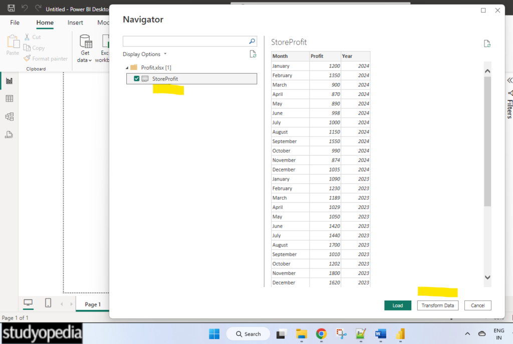
Now, click Load or Transform Data. We will click Transform Data because it will directly take us to the Power Query Editor:
We’ll perform Pivot to get each column as an individual month i.e. the opposite. Therefore, click the Transform tab under the Power Query Editor. To perform the pivot, click the Pivot Column:
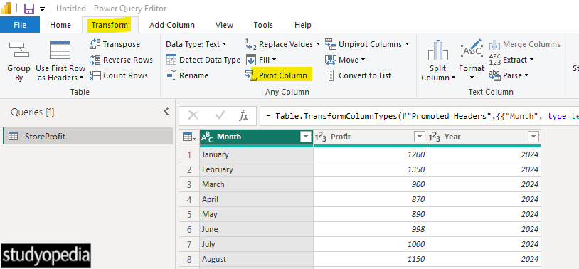
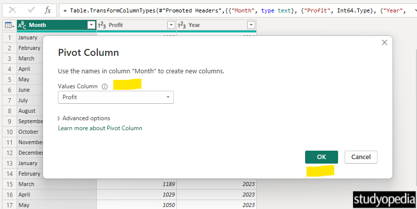
From here, select the Values Column and click Ok. The name and values columns are what we need. The name here is Month and the values Profit:
The pivoted result is now visible. Now, the rows are grouped by years. A separate column for each month can also be seen:
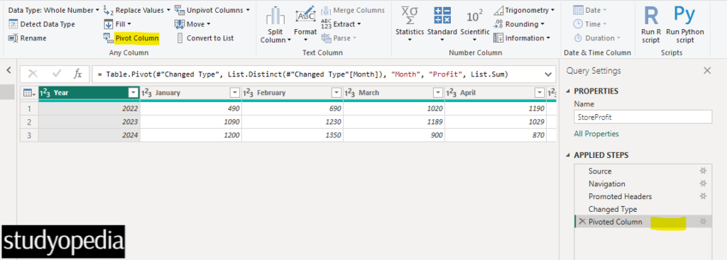
Now, we have the Pivoted Column. On the right, in the Query Settings section, the changes are visible i.e. Pivoted Column under the APPLIED STEPS. If you want to delete, then right-click, and click Delete.
Press CTRL+S and save it:
Video Tutorial
If you don’t want to follow written instructions, you can check out our video tutorial on how to pivot columns in Power BI:
If you liked the tutorial, spread the word and share the link and our website Studyopedia with others.
For Videos, Join Our YouTube Channel: Join Now
Read More:
No Comments