16 May K-Means Clustering Algorithm in Machine Learning
K-Means is a popular unsupervised machine learning algorithm used for clustering tasks. It groups similar data points together into clusters based on their feature similarity, without any prior knowledge of the groups.
Features of K-Means Clustering
The following are the features of K-Means Clustering:
- Unsupervised learning: Doesn’t require labeled data
- Partition-based clustering: Divides data into non-overlapping clusters
- Centroid-based: Each cluster is represented by its center (mean)
- Iterative algorithm: Refines clusters through repeated assignments and centroid updates
How K-Means Works
Let us see how K-Means works:
- Initialize: Randomly select K points as initial centroids
- Assignment: Assign each data point to the nearest centroid
- Update: Recalculate centroids as the mean of all points in each cluster
- Repeat: Steps 2-3 until centroids stabilize or max iterations reached
Advantages of K-Means Clustering
The following are the advantages of K-Means Clustering:
- Simple and easy to implement
- Efficient for large datasets (linear complexity O(n))
- Works well with spherical clusters
- Adapts to new data easily
Disadvantages of K-Means Clustering
The following are the disadvantages of K-Means Clustering:
- Requires pre-specification of K (number of clusters)
- Sensitive to initial centroid selection
- Struggles with non-spherical clusters or varying sizes
- Sensitive to outliers
- Only works well with numerical data
Applications of K-Means Clustering
The following are the applications of K-Means Clustering:
- Customer segmentation
- Image compression (color quantization)
- Document clustering
- Anomaly detection
- Market research
- Social network analysis
Example: K-Means Clustering Python Example with Plot
Step 1: Import the required libraries
import matplotlib.pyplot as plt
from sklearn.datasets import make_blobs
from sklearn.cluster import KMeans
Step 2: Generate sample data
X, y = make_blobs(n_samples=300, centers=4, cluster_std=0.60, random_state=0)
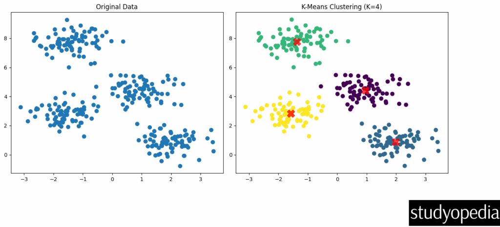
Step 3: Plot the original data
plt.figure(figsize=(12, 5))
plt.subplot(1, 2, 1)
plt.scatter(X[:, 0], X[:, 1], s=50)
plt.title("Original Data")
Step 4: Apply K-Means clustering
kmeans = KMeans(n_clusters=4, random_state=0)
kmeans.fit(X)
y_kmeans = kmeans.predict(X)
Step 5: Plot the clustered data
plt.subplot(1, 2, 2)
plt.scatter(X[:, 0], X[:, 1], c=y_kmeans, s=50, cmap='viridis')
Step 6: Plot the centroids
centers = kmeans.cluster_centers_
plt.scatter(centers[:, 0], centers[:, 1], c='red', s=200, alpha=0.75, marker='X')
plt.title("K-Means Clustering (K=4)")

plt.tight_layout()
plt.show()
Step 7: Print cluster centers
print("Cluster centers:\n", centers)
Output
Displaying cluster centers:

Explanation of the Code
- We generate synthetic data with 4 clusters using make_blobs
- First plot shows the original unlabeled data
- We apply K-Means with K=4 clusters
- Second plot shows the clustered data with colors representing different clusters
- Red X markers show the final cluster centroids
Output Interpretation
- The algorithm successfully identifies the 4 clusters in the data
- Each color represents a different cluster assignment
- The centroids are positioned at the center of each cluster
Determining the Optimal K
A common method to choose K is the elbow method, which looks at the within-cluster sum of squares (WCSS) as a function of K:
wcss = []
for i in range(1, 11):
kmeans = KMeans(n_clusters=i, random_state=0)
kmeans.fit(X)
wcss.append(kmeans.inertia_)

plt.plot(range(1, 11), wcss)
plt.title('Elbow Method')
plt.xlabel('Number of clusters')
plt.ylabel('WCSS')
plt.show()
The “elbow point” where the WCSS starts decreasing linearly indicates a good choice for K.
If you liked the tutorial, spread the word and share the link and our website Studyopedia with others.
For Videos, Join Our YouTube Channel: Join Now
Read More:
No Comments