19 May Keras for Deep Learning
Keras is a high-level, multi-framework deep learning API designed for simplicity and ease of use. In this lesson, we will learn:
- What is Keras?
- Features of Keras
- Advantages of Keras
- Disadvantages of Keras
- Applications of Keras
- Python Keras with Example
What is Keras
Keras is an open-source high-level neural networks API written in Python. It is an interface that runs on top of other frameworks like TensorFlow, Microsoft Cognitive Toolkit (CNTK), or Theano. Since TensorFlow 2.0, Keras has been officially adopted as TensorFlow’s high-level API (tf.keras).
Features of Keras
The following are the features of Keras:
- User-Friendly: Designed for human use with simple, consistent interfaces
- Modular: Neural network layers, cost functions, optimizers, etc. are standalone modules
- Extensible: Easy to add new modules as classes or functions
- Python-based: No separate configuration files needed
- Multi-Backend Support: Works with TensorFlow, Theano, or CNTK
- Multi-Platform: Runs on CPU and GPU
- Built-in Support: For convolutional networks (CNNs), recurrent networks (RNNs), and combinations
Advantages of Keras
The following are the advantages of Keras:
- Easy to learn and use: Great for beginners
- Rapid prototyping: Quickly build and test models
- Large community support: Extensive documentation and tutorials
- Pre-trained models: Access to models like VGG16, ResNet, etc.
- Cross-platform: Can switch between backends
Disadvantages of Keras
The following are the disadvantages of Keras:
- Less flexible: For very custom architectures compared to low-level frameworks
- Performance overhead: Slightly slower than pure TensorFlow/PyTorch for some operations
- Debugging: Can be harder when errors occur in the backend
Applications of Keras
The following are the applications of Keras. Keras is used in:
- Image recognition and classification
- Natural language processing
- Time series forecasting
- Recommendation systems
- Drug discovery
- Game playing AI
Python Keras Example: MNIST Digit Classification
Here’s a complete example of building a simple neural network to classify handwritten digits from the MNIST dataset, with plotting of training history and some sample predictions.
Step 1: Import the required libraries:
|
1 2 3 4 5 6 7 |
import numpy as np import matplotlib.pyplot as plt from tensorflow import keras from tensorflow.keras import layers from tensorflow.keras.datasets import mnist |
Step 2: Load and preprocess data
|
1 2 3 4 5 6 7 |
(x_train, y_train), (x_test, y_test) = mnist.load_data() x_train = x_train.reshape(-1, 28*28).astype("float32") / 255.0 x_test = x_test.reshape(-1, 28*28).astype("float32") / 255.0 y_train = keras.utils.to_categorical(y_train, 10) y_test = keras.utils.to_categorical(y_test, 10) |
Step 3: Build model
|
1 2 3 4 5 6 7 8 9 10 |
model = keras.Sequential([ keras.layers.Input(shape=(784,)), # Explicit Input layer layers.Dense(128, activation='relu'), layers.Dropout(0.2), layers.Dense(64, activation='relu'), layers.Dropout(0.2), layers.Dense(10, activation='softmax') ]) |
Step 4: Compile the model
|
1 2 3 4 5 |
model.compile(optimizer='adam', loss='categorical_crossentropy', metrics=['accuracy']) |
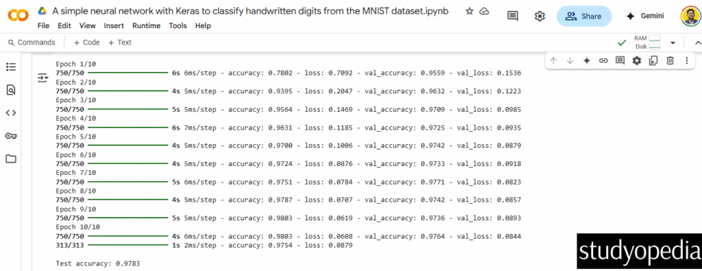
Step 5: Train the model
|
1 2 3 4 5 6 |
history = model.fit(x_train, y_train, batch_size=64, epochs=10, validation_split=0.2) |
Step 6: Evaluate
|
1 2 3 4 |
test_loss, test_acc = model.evaluate(x_test, y_test) print(f"\nTest accuracy: {test_acc:.4f}") |
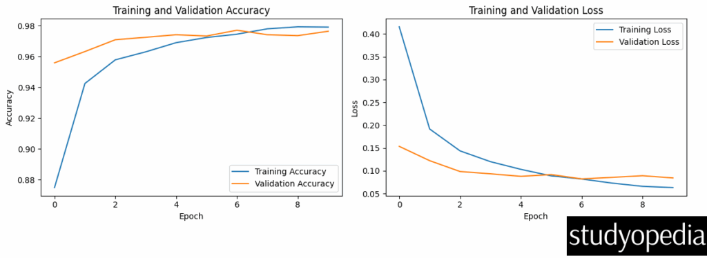
Step 7: Plot training history
|
1 2 3 4 5 6 7 8 9 10 11 12 13 14 15 16 17 18 19 20 21 22 |
plt.figure(figsize=(12, 4)) plt.subplot(1, 2, 1) plt.plot(history.history['accuracy'], label='Training Accuracy') plt.plot(history.history['val_accuracy'], label='Validation Accuracy') plt.title('Training and Validation Accuracy') plt.xlabel('Epoch') plt.ylabel('Accuracy') plt.legend() plt.subplot(1, 2, 2) plt.plot(history.history['loss'], label='Training Loss') plt.plot(history.history['val_loss'], label='Validation Loss') plt.title('Training and Validation Loss') plt.xlabel('Epoch') plt.ylabel('Loss') plt.legend() plt.tight_layout() plt.show() |
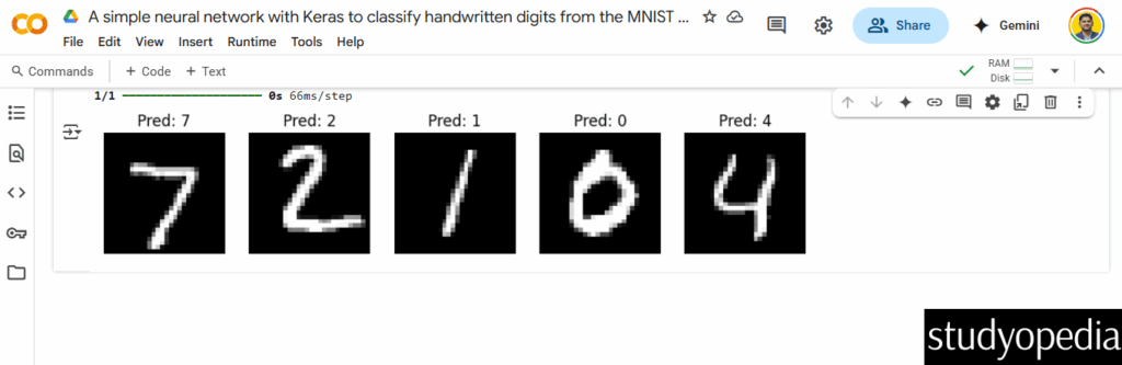
Step 8: Make predictions on some test samples
|
1 2 3 4 5 |
sample_images = x_test[:5].reshape(-1, 28, 28) predictions = model.predict(x_test[:5]) predicted_labels = np.argmax(predictions, axis=1) |
Step 9: Display samples with predictions
|
1 2 3 4 5 6 7 8 9 |
plt.figure(figsize=(10, 2)) for i in range(5): plt.subplot(1, 5, i+1) plt.imshow(sample_images[i], cmap='gray') plt.title(f"Pred: {predicted_labels[i]}") plt.axis('off') plt.show() |
Output
It also shows plots. The first plot will show two graphs side by side:
-
- Left: Training and validation accuracy over epochs
- Right: Training and validation loss over epochs
The second plot will show 5 sample test images with their predicted labels displayed above each image.
If you liked the tutorial, spread the word and share the link and our website Studyopedia with others.
For Videos, Join Our YouTube Channel: Join Now
Read More:
No Comments