19 May TensorFlow for Deep Learning
TensorFlow is a deep learning framework/library that enables developers and researchers to create machine learning models, particularly deep neural networks, with relative ease.
In this lesson, we will learn:
- What is TensorFlow
- Features of TensorFlow
- Advantages of TensorFlow
- Disadvantages of TensorFlow
- Applications of TensorFlow
- Python TensorFlow with Example
What is TensorFlow
TensorFlow is an open-source deep learning framework developed by Google Brain Team. It’s primarily used for machine learning and neural network applications, offering a comprehensive ecosystem of tools, libraries, and community resources.
Features of TensorFlow
The following are the features of TensorFlow:
- Flexibility: Supports both high-level and low-level APIs
- Cross-platform: Runs on CPUs, GPUs, and TPUs
- Scalability: From mobile devices to distributed systems
- Visualization: TensorBoard for model visualization
- Pre-trained models: Access to models through TensorFlow Hub
- Multiple language support: Python (primary), C++, JavaScript, etc.
- Production-ready: Tools for deployment (TF Serving, TF Lite, TF.js)
Advantages of TensorFlow
The following are the advantages of TensorFlow:
- Comprehensive ecosystem: Tools for every stage of ML workflow
- Production deployment: Excellent support for deploying models
- Community support: Large, active community
- Visualization: TensorBoard provides excellent model insights
- Google support: Backed by Google with regular updates
Disadvantages of TensorFlow
The following are the disadvantages of TensorFlow:
- Steep learning curve: Especially for beginners
- Verbose syntax: Can be more verbose than some alternatives
- Performance overhead: Some operations can be slower than PyTorch
- Static computation graph: Though eager execution helps (enabled by default in TF 2.x)
Applications of TensorFlow
The following are the applications of TensorFlow:
- Image and video recognition
- Natural language processing
- Time series analysis
- Recommendation systems
- Generative models (GANs, VAEs)
- Reinforcement learning
- Medical image analysis
Python TensorFlow Example with Plot
Step 1: Import the required libraries:
import numpy as np
import matplotlib.pyplot as plt
import tensorflow as tf
from tensorflow.keras import layers, models, Input
Step 2: Generate synthetic data
np.random.seed(42)
X = np.linspace(-1, 1, 100)
y = 2 * X + 1 + np.random.normal(0, 0.2, 100)
Step 3: Split data into train and test
X_train, y_train = X[:80], y[:80]
X_test, y_test = X[80:], y[80:]
Step 4: Build a simple sequential model with proper Input layer
model = models.Sequential([
Input(shape=(1,)), # Proper way to specify input shape
layers.Dense(64, activation='relu'),
layers.Dense(64, activation='relu'),
layers.Dense(1)
])
Step 5: Compile the model
model.compile(optimizer='adam',
loss='mse',
metrics=['mae'])
Step 6: Train the model with early stopping
callback = tf.keras.callbacks.EarlyStopping(monitor='val_loss', patience=10)
history = model.fit(X_train, y_train,
epochs=200, # Increased epochs since we have early stopping
batch_size=8,
validation_split=0.2,
callbacks=[callback],
verbose=0)
Step 7: Evaluate the model
test_loss, test_mae = model.evaluate(X_test, y_test, verbose=0)
print(f"Test MAE: {test_mae:.4f}")
Step 8: Make predictions
y_pred = model.predict(X_test)
Step 9: Plot training history
plt.figure(figsize=(12, 5))

plt.subplot(1, 2, 1)
plt.plot(history.history['mae'], label='Training MAE')
plt.plot(history.history['val_mae'], label='Validation MAE')
plt.xlabel('Epoch')
plt.ylabel('MAE')
plt.title('Training and Validation MAE')
plt.legend()
Step 10: Plot predictions vs actual
plt.subplot(1, 2, 2)
plt.scatter(X_train, y_train, label='Training data', alpha=0.6)
plt.scatter(X_test, y_test, label='Test data', alpha=0.6)
plt.plot(X_test, y_pred, 'r-', label='Predictions', linewidth=2)
plt.xlabel('X')
plt.ylabel('y')
plt.title('Model Predictions vs Actual Data')
plt.legend()

plt.tight_layout()
plt.show()
Output
It displays the following output.
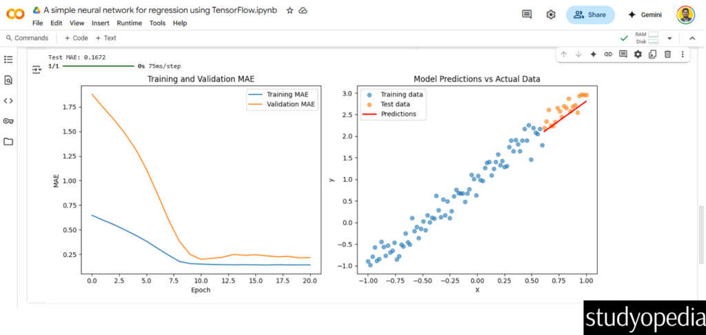
Test MAE: 0.1932
Here are the output two plots:
- Training history showing MAE decreasing over epochs. Another one is the:
- Predictions vs actual data showing how well the model fits
Here is the output:
If you liked the tutorial, spread the word and share the link and our website Studyopedia with others.
For Videos, Join Our YouTube Channel: Join Now
Read More:
No Comments