19 May PyTorch for Deep Learning
PyTorch is a deep learning framework/library that has gained tremendous popularity in both research and production environments. In this lesson, we will learn:
- What is PyTorch
- Features of PyTorch
- Advantages of PyTorch
- Disadvantages of PyTorch
- Applications of PyTorch
- Python PyTorchwith Example
What is PyTorch
PyTorch is an open-source machine learning library primarily used for deep learning applications. Developed by Facebook’s AI Research lab (now Meta AI), it provides a flexible and intuitive platform for building and training neural networks.
Features of PyTorch
The following are the features of PyTorch:
- Dynamic Computation Graphs: Uses dynamic computation graphs (define-by-run) through its autograd system, allowing for more flexible model architectures.
- GPU Acceleration: Provides seamless CPU/GPU switching with CUDA support for accelerated computing.
- Pythonic Nature: Feels more “native” to Python developers compared to other frameworks.
- TorchScript: Allows models to be serialized and optimized for production deployment.
- Distributed Training: Supports data parallelism and model parallelism for large-scale training.
- Rich Ecosystem: Includes tools like TorchVision, TorchText, and TorchAudio for specific domains.
- Automatic Differentiation: Built-in autograd system handles gradient computation automatically.
Advantages of PyTorch
The following are the advantages of PyTorch:
- Ease of Use: More intuitive and pythonic than many alternatives
- Debugging: Easier to debug due to imperative programming style
- Research Friendly: Rapid prototyping capabilities
- Community: Strong and growing community support
- Deployment: Good options for production deployment
Disadvantages of PyTorch
The following are the disadvantages of PyTorch:
- Production Readiness: Historically lagged behind TensorFlow (though this gap has narrowed)
- Mobile Support: Not as robust as some competitors for mobile deployment
- Visualization: Requires additional tools like TensorBoard or Weights & Biases
Applications of PyTorch
PyTorch is used across various domains:
- Computer Vision (image classification, object detection)
- Natural Language Processing (translation, text generation)
- Reinforcement Learning
- Time Series Analysis
- Generative Models (GANs, VAEs)
- Scientific Computing
PyTorch Example with Plot
Here’s a complete example of training a simple neural network on synthetic data with plotting:
Step 1: Import the required libraries
import torch
import torch.nn as nn
import torch.optim as optim
import numpy as np
import matplotlib.pyplot as plt
from sklearn.datasets import make_moons
from sklearn.model_selection import train_test_split
Step 2: Set random seeds for reproducibility
torch.manual_seed(42)
np.random.seed(42)
Step 3: Generate synthetic data (two interleaving half circles)
X, y = make_moons(n_samples=1000, noise=0.1, random_state=42)
X = X.astype(np.float32)
y = y.astype(np.float32)
Step 4: Split into train and test sets
X_train, X_test, y_train, y_test = train_test_split(X, y, test_size=0.2, random_state=42)
Step 5: Convert to PyTorch tensors
X_train_tensor = torch.from_numpy(X_train)
y_train_tensor = torch.from_numpy(y_train).view(-1, 1)
X_test_tensor = torch.from_numpy(X_test)
y_test_tensor = torch.from_numpy(y_test).view(-1, 1)
Step 6: Define a simple neural network
class MoonClassifier(nn.Module):
def __init__(self):
super(MoonClassifier, self).__init__()
self.layer1 = nn.Linear(2, 16)
self.layer2 = nn.Linear(16, 16)
self.output = nn.Linear(16, 1)
self.relu = nn.ReLU()
self.sigmoid = nn.Sigmoid()

def forward(self, x):
x = self.relu(self.layer1(x))
x = self.relu(self.layer2(x))
x = self.sigmoid(self.output(x))
return x
Step 7: Initialize model, loss function, and optimizer
model = MoonClassifier()
criterion = nn.BCELoss() # Binary Cross Entropy Loss
optimizer = optim.Adam(model.parameters(), lr=0.01)
Step 8: Training loop
epochs = 500
train_losses = []
test_losses = []

for epoch in range(epochs):

# training
model.train()
optimizer.zero_grad()
outputs = model(X_train_tensor)
loss = criterion(outputs, y_train_tensor)
loss.backward()
optimizer.step()
train_losses.append(loss.item())
Step 9: Testing
model.eval()
with torch.no_grad():
test_outputs = model(X_test_tensor)
test_loss = criterion(test_outputs, y_test_tensor)
test_losses.append(test_loss.item())
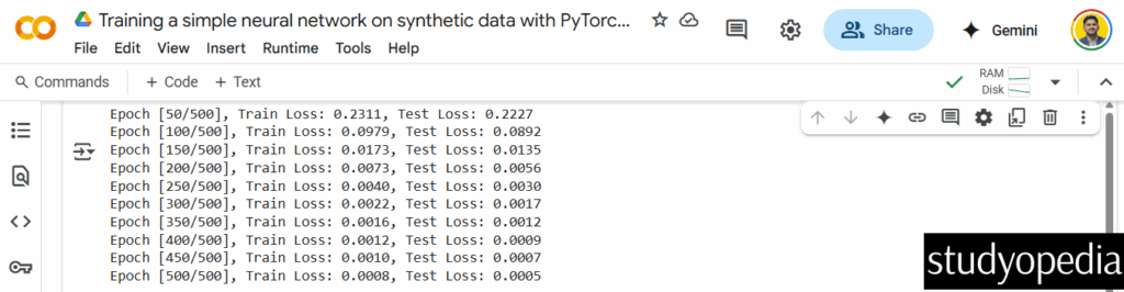
if (epoch+1) % 50 == 0:
print(f'Epoch [{epoch+1}/{epochs}], Train Loss: {loss.item():.4f}, Test Loss: {test_loss.item():.4f}')
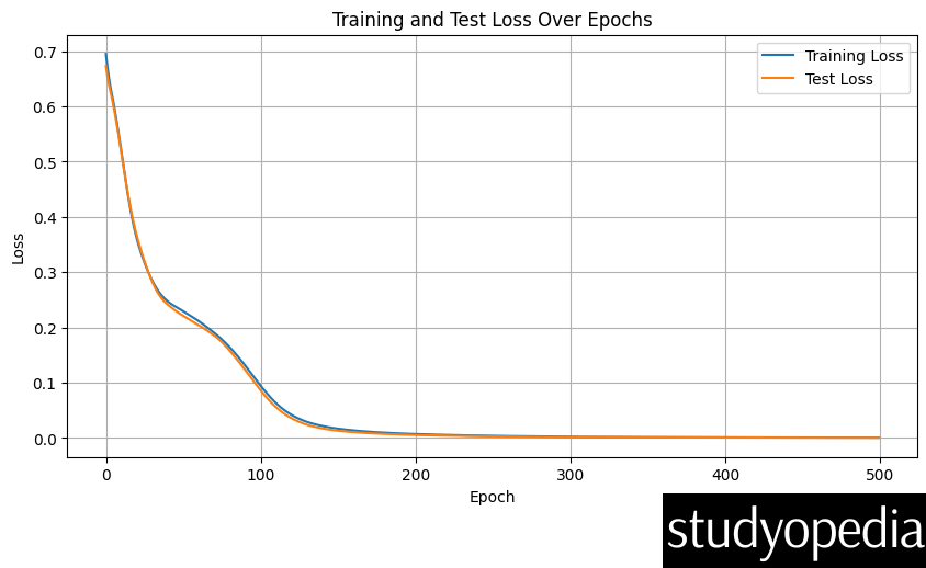
Step 10: Plot the training and test loss
plt.figure(figsize=(10, 5))
plt.plot(train_losses, label='Training Loss')
plt.plot(test_losses, label='Test Loss')
plt.title('Training and Test Loss Over Epochs')
plt.xlabel('Epoch')
plt.ylabel('Loss')
plt.legend()
plt.grid(True)
plt.show()
Step 11: Create a mesh grid for visualization
x_min, x_max = X[:, 0].min() - 0.5, X[:, 0].max() + 0.5
y_min, y_max = X[:, 1].min() - 0.5, X[:, 1].max() + 0.5
xx, yy = np.meshgrid(np.linspace(x_min, x_max, 100),
np.linspace(y_min, y_max, 100))
Step 12: Predict on mesh grid
model.eval()
with torch.no_grad():
Z = model(torch.tensor(np.c_[xx.ravel(), yy.ravel()], dtype=torch.float32))
Z = Z.view(xx.shape).numpy()
Step 13: Plot decision boundary and data points
plt.figure(figsize=(10, 8))
plt.contourf(xx, yy, Z > 0.5, alpha=0.3)
plt.scatter(X[:, 0], X[:, 1], c=y, edgecolors='k', cmap=plt.cm.Paired)
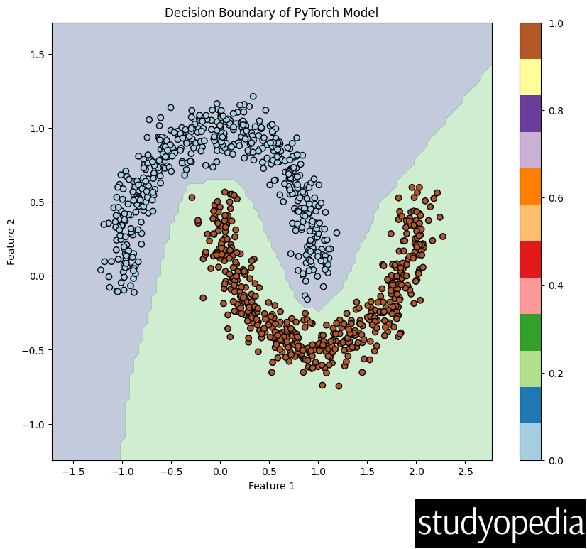
plt.title('Decision Boundary of PyTorch Model')
plt.xlabel('Feature 1')
plt.ylabel('Feature 2')
plt.colorbar()
plt.show()
Output
Here is the output:
The code produces two plots:
Loss Curve Plot: Shows the training and test loss decreasing over epochs, indicating the model is learning:
Decision Boundary Plot: Visualizes how the neural network has learned to separate the two classes (the moons) in the 2D feature space:
The example demonstrates:
- Creating a neural network in PyTorch
- Training loop with loss calculation and backpropagation
- Model evaluation
- Visualization of results
- Handling of synthetic data
The model achieves good separation of the two moon-shaped classes, showing PyTorch’s capability to learn non-linear decision boundaries.
PyTorch’s flexibility makes it excellent for such prototyping tasks while also scaling well to larger, more complex problems.
If you liked the tutorial, spread the word and share the link and our website Studyopedia with others.
For Videos, Join Our YouTube Channel: Join Now
Read More:
No Comments